ADS-B evaluation dataset
The ADS-B evaluation dataset included in ContrailBench provides a gridded dataset of flight distance based on global ADS-B telemetry. Although this dataset does not provide information about contrail formation, it is used for metrics related to the cost of contrail avoidance (e.g., flight distance within forecast contrail regions). See preprocess_adsb.py for details on how this data is prepared from ADS-B telemetry.
The ADS-B evaluation dataset is available alongside other evaluation datasets in a public cloud bucket (gs://contrailbench-public-data). This notebook shows
How to load ADS-B evaluation data using Pandas
How to interpret the contents of the ADS-B evaluation dataset
How to use the ADS-B evaluation dataset to compute ContrailBench cost metrics
[1]:
import datetime
import os

import aiohttp
import cartopy.crs as ccrs
import matplotlib.pyplot as plt
import numpy as np
import pandas as pd
import xarray as xr
from matplotlib import colors
Loading ADS-B evaluation data
ADS-B evaluation data is sharded by time (one file per hour) and altitude (one file per flight level). Coverage for each ContrailBench release cycle is as follows:
Release |
Times |
Altitudes |
GCS path |
|---|---|---|---|
v1 |
Jan-Dec 2024 |
FL270-440 |
|
Because gridded ADS-B data is relatively sparse, the dataset is stored as parquet files with one row for each grid cell with non-zero flight distance. These files can be read directly from GCS with Pandas.
Warning: be very careful about timezone-naive datetimes when using ContrailBench evaluation datasets. Python’s datetime module assumes that naive datetimes represent local time, which affects the POSIX timestamp returned by
datetime.timestamp().
[2]:
gcs_path = "gs://contrailbench-public-data/v1/adsb"
time = datetime.datetime(2024, 6, 1, 0, tzinfo=datetime.UTC)
flight_level = 350

df = pd.read_parquet(f"{gcs_path}/{int(time.timestamp())}_{flight_level}.pq")
df
[2]:
| longitude | latitude | flight_distance | |
|---|---|---|---|
| 0 | -180.00 | 24.00 | 26008.575795 |
| 1 | -180.00 | 57.00 | 18297.307009 |
| 2 | -179.75 | 24.00 | 25715.243743 |
| 3 | -179.75 | 57.00 | 15665.218763 |
| 4 | -179.50 | 24.00 | 23377.388211 |
| ... | ... | ... | ... |
| 27699 | 179.50 | 24.00 | 18919.963119 |
| 27700 | 179.50 | 56.75 | 5217.623015 |
| 27701 | 179.50 | 57.00 | 10453.280407 |
| 27702 | 179.75 | 24.00 | 26013.218937 |
| 27703 | 179.75 | 57.00 | 15702.158910 |
27704 rows × 3 columns
Interpretation
Rows of the dataset provide total flight distance (in meters) aggregated on a spatiotemporal grid with 0.25 degree horizontal resolution. Horizontal bounds are from -180 degrees to 179.75 degrees longitude and -80 degrees to 80 degrees latitude. The total flight distance within a grid cell includes all flight segments
within 0.125 degrees latitude and longitude of the provided latitude and longitude coordinates,
within 250 vertical ft of the target flight level, and
within 30 minutes of the target time
Grid cells with zero flight distance are omitted from the dataset to reduce data volume. If necessary, they can be restored using xarray:
[3]:
all_lons = np.arange(-180.0, 180.0, 0.25)
all_lats = np.arange(-80, 80.25, 0.25)
ds = df.set_index(["longitude", "latitude"]).to_xarray().fillna(0.0)
ds = ds.reindex(longitude=all_lons, latitude=all_lats, fill_value=0.0)
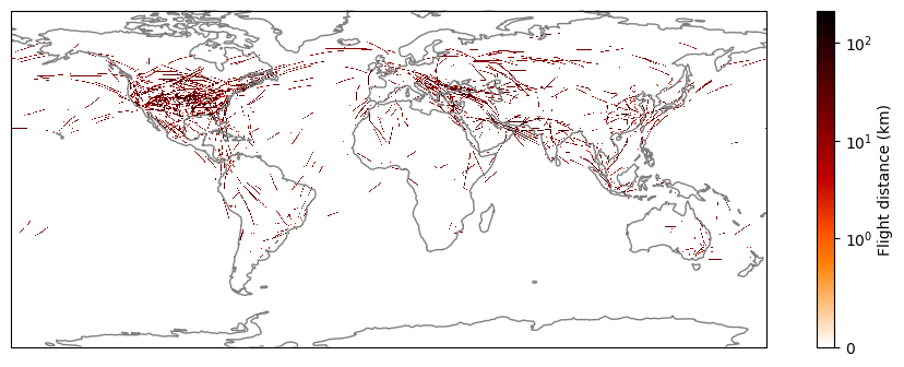
[4]:
plt.figure(figsize=(12, 4))
ax = plt.subplot(111, projection=ccrs.PlateCarree())
im = ax.pcolormesh(
    ds["longitude"],
    ds["latitude"],
    ds["flight_distance"].T / 1e3,
    shading="nearest",
    cmap="gist_heat_r",
    norm=colors.SymLogNorm(linthresh=1, vmin=0),
    transform=ccrs.PlateCarree(),
)
plt.colorbar(im, ax=ax, label="Flight distance (km)")
ax.coastlines(color="gray");
Use in ContrailBench metrics
The ADS-B evaluation dataset is used in PCR benchmarks to calculate the fraction of global flight distance through forecast contrail regions, a proxy for the cost of contrail avoidance.
This notebook uses the Contrails.org forecast for an example calculation. See the Contrails.org example notebook for details about accessing and preprocessing the Contrails.org forecast.
[5]:
url = "https://api.contrails.org/v1/grids"
params = {
    "aircraft_class": "default",
    "flight_level": str(flight_level),
    "time": time.strftime("%Y-%m-%dT%H"),
    "units": "ef_per_m",
}
headers = {"x-api-key": os.environ["CONTRAILS_API_KEY"]}

async with (
    aiohttp.ClientSession(raise_for_status=True) as session,
    session.get(url, params=params, headers=headers) as resp,
):
    content = await resp.read()

with open("forecast.nc", "wb") as f:
    f.write(content)
ds = xr.open_dataset("forecast.nc")

ds["pcr"] = ds["ef_per_m"] != 0
processed = ds[["pcr"]]
The fraction of flight distance inside forecast PCRs can be calculated using some xarray indexing tricks.
[6]:
target_lon = xr.DataArray(df["longitude"], dims="row")
target_lat = xr.DataArray(df["latitude"], dims="row")
flight_dist = xr.DataArray(df["flight_distance"], dims="row")

pcr = processed["pcr"].sel(longitude=target_lon, latitude=target_lat)
pcr_dist = flight_dist.where(pcr).sum().item()
tot_dist = flight_dist.sum().item()

print(f"Fraction of flight distance inside forecast PCRs: {pcr_dist / tot_dist:.3f}")
Fraction of flight distance inside forecast PCRs: 0.086